Backpropagation

Backpropagation computes the gradient of the loss with respect to every parameter in the network by applying the Chain Rule (Multivariable) on the computation graph.

Forward pass: compute output layer by layer, storing all intermediates.

Backward pass: propagate gradients from loss backward:

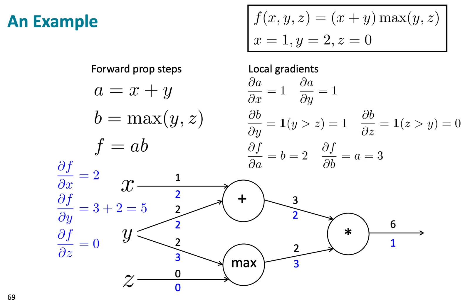
Each node receives an upstream gradient and passes down a downstream gradient = upstream × local gradient, where the local gradient is the gradient of the node's output w.r.t. its input. Backprop visits nodes in reverse topological order, seeding the output gradient with $\partial L/\partial L = 1$.

Gate intuitions:

• $+$ distributes the upstream gradient unchanged to each summand
• $\max$ routes the upstream gradient to whichever input was largest
• $\times$ swaps the forward inputs as coefficients on the downstream gradient
• gradients sum at outward branches: if $y$ feeds both $a$ and $b$, then $\frac{\partial f}{\partial y} = \frac{\partial f}{\partial a}\frac{\partial a}{\partial y} + \frac{\partial f}{\partial b}\frac{\partial b}{\partial y}$

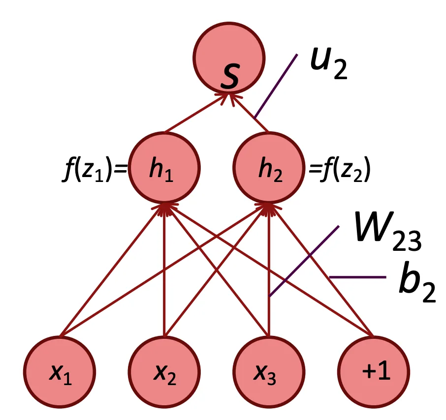
For a 2-layer MLP with $\mathbf{h} = \sigma(W_1\mathbf{x})$, $\hat{y} = W_2\mathbf{h}$, $L = \frac{1}{2}\|\hat{y} - y\|^2$:

1. $\frac{\partial L}{\partial \hat{y}} = \hat{y} - y$
2. $\frac{\partial L}{\partial W_2} = \frac{\partial L}{\partial \hat{y}} \cdot \mathbf{h}^\top$
3. $\frac{\partial L}{\partial \mathbf{h}} = W_2^\top \frac{\partial L}{\partial \hat{y}}$
4. $\frac{\partial L}{\partial W_1} = \left(\frac{\partial L}{\partial \mathbf{h}} \odot \sigma'(W_1\mathbf{x})\right) \cdot \mathbf{x}^\top$

Vanishing gradients: if $|\sigma'| < 1$ consistently (sigmoid), gradients shrink exponentially with depth. Solutions:

• ReLU — gradient is 1 for positive inputs
• Residual Connections — gradient highway that bypasses layers
• Weight Initialization — controls initial gradient magnitudes
• Batch Normalization — stabilizes intermediate distributions

Gradient checking: verify a hand-derived gradient against a numerical estimate using the symmetric difference $f'(x) \approx \frac{f(x+h) - f(x-h)}{2h}$.

Activation / gradient checkpointing trades compute for memory: store only a subset of activations (the "checkpoints") and recompute the rest on the fly during the backward pass. For $N$ layers split into $K$ segments, memory drops from $O(N)$ to $O(K + N/K)$; the optimum $K = \sqrt{N}$ gives $O(\sqrt{N})$ memory at the cost of one extra forward pass ($\sim 2N$ backward compute).

In PyTorch: loss.backward() traverses the computation graph and populates .grad for every parameter. optimizer.step() then applies SGD/Adam. Backprop must start from a scalar loss, since $\partial L/\partial \theta$ is one number per parameter; with mean reduction, by linearity the batch gradient is exactly the mean of per-example gradients.

See also: The Artificial Neuron, Computation Graphs