Transformers and LLMs

Transformers and LLMs model token sequences by repeatedly mixing contextual information across positions. The useful mental model is: tokenization creates discrete symbols, attention moves information between symbols, and autoregressive training turns next-token prediction into a scalable learning signal.

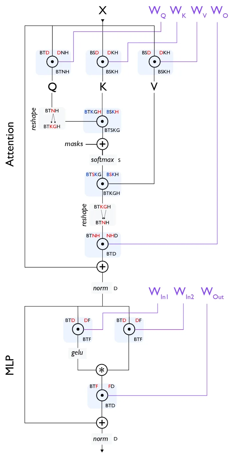
Dimension conventions (used across the architecture):

A modern decoder block is: RMSNorm → attention (with RoPE, GQA) → residual → RMSNorm → SwiGLU FFN → residual. Parameter count is $\approx 2VD + 12LD^2$.

Core sequence:

1. Tokenization - maps text into discrete tokens that the model can embed.
2. Autoregressive Generation - generates one token at a time conditioned on previous tokens.
3. Positional Encoding - gives the model access to order because attention alone is permutation-equivariant.
4. Self-Attention - lets each token read from other tokens.
5. Multi-Head Attention - runs several attention subspaces in parallel.
6. Causal Masking - prevents positions from attending to future tokens during autoregressive training.
7. Computational Complexity of Attention - explains the $O(n^2)$ sequence-length bottleneck.
8. Pretraining - trains broad capability from large-scale next-token prediction.
9. Scaling Laws - describes empirical relationships among data, parameters, compute, and loss.
10. Sampling and Decoding Strategies - controls generation from model probabilities.
11. Supervised Fine-Tuning - adapts a pretrained model to demonstrations of desired behavior.
12. LoRA - fine-tunes low-rank adapter matrices instead of all weights.
13. RLHF Pipeline - trains against human preferences through a reward model and policy optimization.
14. KL Penalty - constrains policy updates away from a reference model.
15. Direct Preference Optimization - optimizes preferences without an explicit reward model.
16. Chain-of-Thought Prompting - elicits intermediate reasoning tokens.
17. ReAct - interleaves reasoning and tool actions.
18. Test-Time Compute - spends more inference compute for better answers.
19. Self-Improvement in LLMs - studies model-generated data, feedback, and iterative improvement loops.
20. LLMs as RL Agents - views language models as policies acting through text or tools.

How the pieces fit:

• Tokenization and embeddings define the input representation.
• Positional encoding, self-attention, multi-head attention, and causal masks define the transformer block's sequence computation.
• Complexity analysis explains why long context is expensive.
• Pretraining and scaling laws explain why next-token prediction can produce broad competence.
• Sampling controls behavior at inference time.
• SFT, LoRA, RLHF, KL penalties, and DPO are post-training methods.
• Chain-of-thought, ReAct, test-time compute, and self-improvement concern inference-time or iterative behavior.

Core equations to keep active:

• Autoregressive factorization: $p(x_{1:T}) = \prod_{t=1}^T p(x_t|x_{<t})$
• Attention: $\mathrm{Attention}(Q,K,V) = \mathrm{softmax}\left(\frac{QK^\top}{\sqrt{d_k}}\right)V$
• Causal mask: set attention logits to $-\infty$ for future positions.
• Pretraining loss: $L = -\sum_t \log p_\theta(x_t|x_{<t})$
• Attention complexity: standard self-attention costs $O(n^2 d)$ in sequence length $n$.
• LoRA update: $W' = W + BA$ with low-rank $A,B$.
• KL-regularized objective: $\mathbb{E}[R(x,y)] - \beta D_{\mathrm{KL}}(\pi_\theta(\cdot|x) \| \pi_{\mathrm{ref}}(\cdot|x))$
• DPO preference term: $\log \sigma\left(\beta\left[\log\frac{\pi_\theta(y_w|x)}{\pi_{\mathrm{ref}}(y_w|x)} - \log\frac{\pi_\theta(y_l|x)}{\pi_{\mathrm{ref}}(y_l|x)}\right]\right)$

See also: Neural Networks, Reinforcement Learning, Systems and Scaling